2. Transformer Development #

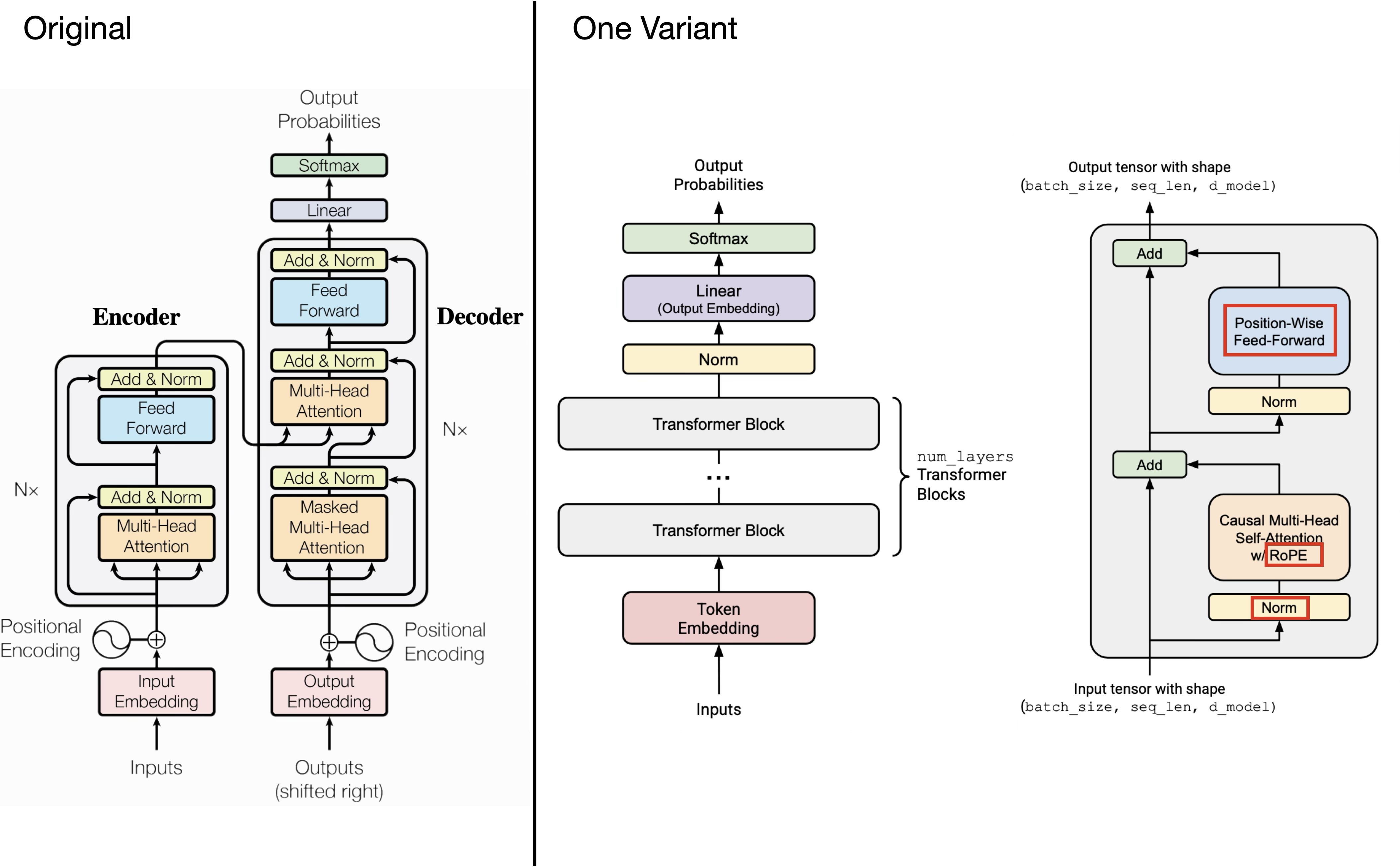
1. Original Transformer #

Steps:

• $\operatorname{FFN}\left(\tilde{z}^{l}\right)=\max \left(0, \tilde{z}^{l} W 1+b 1\right) W 2+b 2$

1. Input embeddings: $ z^0 = E(x) + PE $, positional enocding: sines and cosines

2. Encoder (repeat $N$ times):

3. Decoder input: $y^0 = E(y) + PE, \quad y=(\langle\mathrm{sos}\rangle, y 1, y 2, \ldots, y T-1)$

4. Decoder (repeat $N$ times):

5. Output layer:

2. Architecture variations #

1. use prenorm instead of postnorm: keep the good parts of residual connections; make the training more stable,no need to warm up

• $y=x+$ MHA(RMSNorm($x$)), $y=y+$ SwiGLU(RMSNorm(y))
• use double norm: (some architecutres) LN -> MAH/FNN ->LN

2. use RMSNorm instead of LayerNorm: fewer operations, less memory movement

1. LayerNorm – normalizes the mean and variance across $𝑑_{𝑚𝑜𝑑𝑒𝑙}$: $y=\frac{x-\mathrm{E}[x]}{\sqrt{\operatorname{Var}[x]+\epsilon}} * \gamma+\beta$
2. RMSNorm: no mean subtraction/bias: $y=\frac{x}{\sqrt{||x||_{2}^{2}+\varepsilon}} * \gamma$

3.FFN: No Bias Term: memory (similar to RMSnorm) and optimization stability

1. original: $\operatorname{FFN}(x)=\max \left(0, x W_{1}+b_{1}\right) W_{2}+b_{2}$
2. most(if not gated): $FFN(x)=\sigma\left(x W_{1}\right) W_{2}$

4. Gated Activation

1. ReLU: $F F(x)=\max \left(0, x W_{1}\right) W_{2}$
2. GeLU: $F F(x)=\operatorname{GELU}\left(x W_{1}\right) W_{2},\quad G E L U(x):=x \Phi(x)$
3. modern: Gated activations: Instead of a linear + ReLU, augment the above with an (entrywise) linear term. Gated models use smaller dimensions for the $d_{f f}$ by $2 / 3$.
   • $FFN_{\text{ReGLU}}(x)=\left(\max \left(0, x W_{1}\right) \otimes x V\right) W_{2}$
   • $FFN_{\text{GEGLU}}\left(x, W, V, W_{2}\right)=(\text{GELU}(x W) \otimes x V) W_{2}$

4. SwiGLU (swish is $x * \operatorname{sigmoid}(x)$ )
   • $FFN_{\text {SwiGLU }}\left(x, W, V, W_{2}\right)=\left(Swish_{1}(x W) \otimes x V\right) W_{2}$

5. Serial instead of Parallel Layers

• Parallel: $y=x+\operatorname{FFN}(\operatorname{Norm}(x))+\operatorname{Attention}(\operatorname{Norm}(x))$
• Serial: $y=x+\operatorname{FFN}(\operatorname{Norm}(x+\operatorname{Attention}(\operatorname{Norm}(x)))$

6. Position EMbedding: use ROPE for relative embedding, implement at attention layer for Q, K

3. Hyperparameters #

1. FF(RELU):$d_{f f}=4 d_{\text {model }}$, gated: FF(GLU): $d_{f f}=\frac{8}{3} d_{\text {model }}$
2. $d_{head}*h=d_{model}$
3. aspect ratio: $d_{\text {model }} / n_{\text {layer }}\approx 100$
4. vocabulary size: monolingual models - 30-50k, Multilingual: 100-250k

4. Regularzation #

• becuase of large data, there is not a big issue on overfitting

1. weight decay is interacting with learning rate schedule(cosine schedule) to improve the tranining, not due to regularization
2. don’t need to do droupout

5. Stability tricks #

1. softmax: 1) before the output probability, and 2) in attention

   1. • softmax= $\log (P(x))=\log \left(\frac{e^{U_{r}(x)}}{Z(x)}\right)=U_{r}(x)-\log (Z(x))$, $Z(x)=\Sigma_{r^{\prime}=1}^{|V|} e^{U_{r^{\prime}}(x)}$
   • we want to make z(x) close to 1: so modify the loss function: $$ L=\sum\left[\log \left(P\left(x_{i}\right)\right)-\alpha\left(\log \left(Z\left(x_{i}\right)\right)-0\right)^{2}\right] $$
   2. normalize Q,K before attention
   3. Use more layernorm
   4. Soft-capping the logits to some maximum value via Tanh:
   • logits $\leftarrow$ soft_cap $*$ tanh (logits/soft_cap)

6. Attention Heads #

GQA/MQA - Redudcing attention head cost

• grouped query attention, multi query attention
• artihmetic intensity is high

At training

1. Arithmetic(FLOPS) calculation:

• $b$: batch size, $n$: sequence length, $d$: model width, $h$: #heads, $d_h=d/h$.
• Input $X\in\mathbb{R}^{b\times n\times d}$.
• Rule of thumb for a matmul: $(m\times n)\cdot(n\times p)$ costs $\approx 2mnp$ FLOPs.

  1. Linear projections $Q=XW_Q,;K=XW_K,;V=XW_V,;O=\text{concat heads}\cdot W_O$. Each is $(bn\times d)\cdot(d\times d)\Rightarrow \approx 2,bn,d^2$ FLOPs.

  2. Attention scores and mixing (per head) $S_t=Q_tK_{\pi(t)}^\top \in \mathbb{R}^{b\times n\times n}$: $(bn\times d_h)\cdot(d_h\times n) \Rightarrow 2,bn,n,d_h$. Across $h$ heads: $2,bn,n,h,d_h=2,bn^2d$.

  3. Mixing $O_t=\mathrm{softmax}(S_t)V_{\pi(t)}$ is the same cost again: $2,bn^2d$.

     $$ \boxed{\text{Arithmetic}}=\underbrace{8\,bn\,d^2}_{\text{4 projections}} \;+\; \underbrace{4\,bn^2d}_{\text{scores+mix}} \sim O(b n d^{2})$$

2. Memory accesses (reads/writes)

   1. Activations scale ($bnd$): Reading $X$ / writing outputs / intermediate tensors are all $\Theta(bnd)$.

   2. Attention maps ($bhn^2$): For each batch and head you materialize (or at least stream) an $n\times n$ score/probability tile for softmax/mixing.

   3. Weights ($d^2$): Loading the dense projection weights $W_Q,W_K,W_V,W_O$ is $\Theta(d^2)$.

      $$ \boxed{\text{Memory } \sim\; bnd \;+\; bhn^2 \;+\; d^2 }. $$
3. Arithmetic intensity
   • $\mathrm{AI} \sim \frac{b n d^{2}}{d^{2}+b n d+b g n^{2}}\sim \frac{1}{b n}+\frac{1}{k}+$ smaller terms
   • High AI ⇒ each byte loaded from memory is reused many times in math ⇒ compute-bound (GPU fully busy)

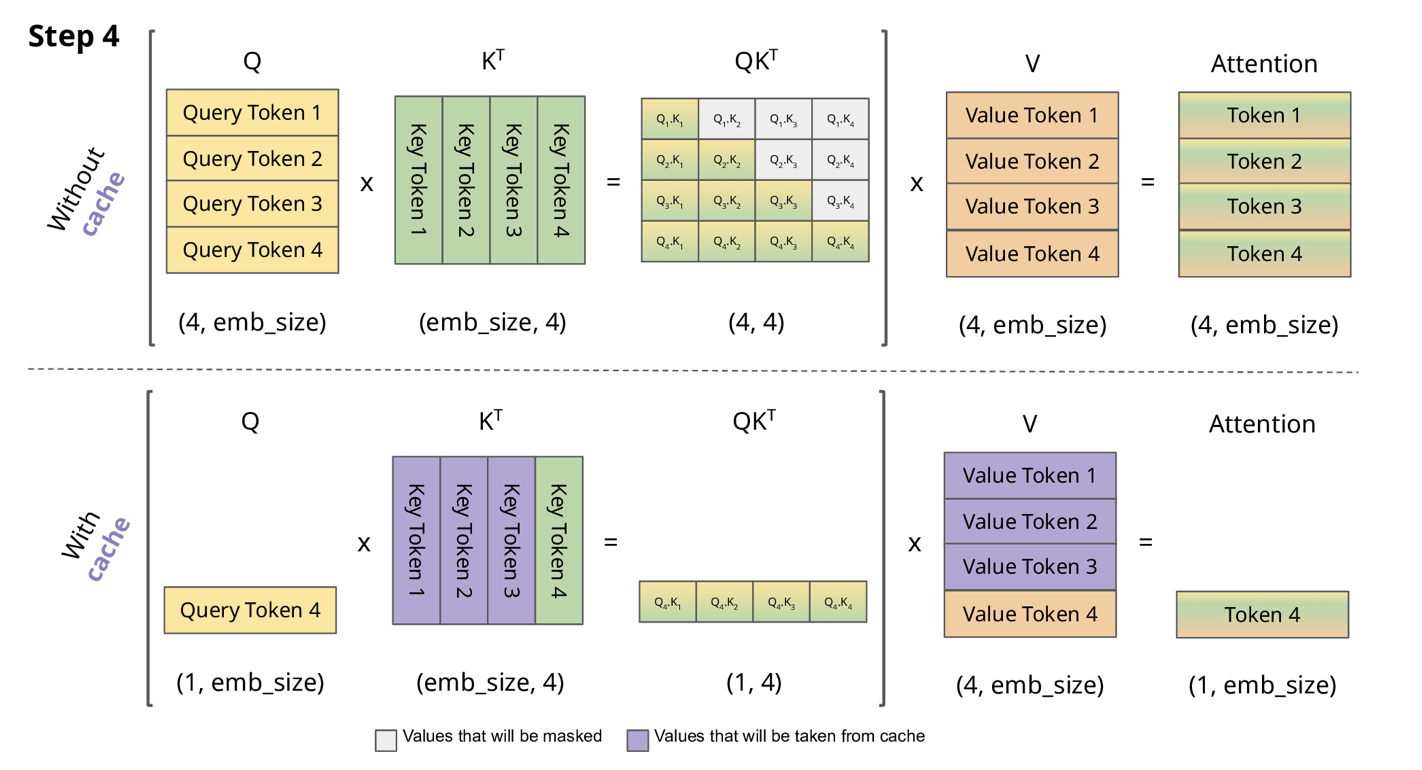
At inference: we need to incrementaly re-compute/update attention via the ‘KV cache’

(Picture from KV Caching@joaolages )

1. Total arithmetric operations $\left(b n d^{2}\right)$, total memory accesses $\left(b n^{2} d+n d^{2}\right)$
2. Arithmetic intensity is not good $O\left(\left(\frac{n}{d}+\frac{1}{b}\right)^{-1}\right)$ - need large batches + short seq length (n) or big model dimensions (d)

tbd

Step details #

0: Tokenization #

Before embeddings, raw text must be converted into token IDs.

1. Text input: Example: "I like AI"

2. Tokenizer:

   • Splits text into units (tokens). Can be word-level, subword-level (BPE/WordPiece), or character-level.
   • Each token is mapped to an integer ID from the vocabulary.

   Example (WordPiece): "I like AI" → ["I", "like", "AI"]

3. Token IDs: ["I", "like", "AI"] → [101, 456, 982]

   • $101, 456, 982$ are indices into the vocabulary of size $V$.
   • Each ID uniquely represents a token.

4. Results: $ \text{Token IDs} \in \mathbb{Z}^{B \times T}$,

   • $B$ is batch size, $T$ is sequence length.

1: Token IDs → Embedding Vectors #

1. Embedding matrix: A learnable parameter $ E \in \mathbb{R}^{V \times d_{\text{model}}}$

   • $V$: vocabulary size (e.g., 30,000)
   • $d_{\text{model}}$: hidden dimension (e.g., 512, 768, 1024)

2. Lookup: For each token ID $t_i$, fetch its row in $E$: $ x_i = E[t_i] \in \mathbb{R}^{d_{\text{model}}} $

3. Stack into batch: $ X \in \mathbb{R}^{B \times T \times d_{\text{model}}} $

   • $X[b, i, :]$: embedding for the $i$-th token in the $b$-th sequence.

2. Linear Projections for Q, K, V #

• Each token vector is projected into query, key, and value spaces.

• For multi-head attention with $h$ heads:

  $$ Q = X W^Q, \quad K = X W^K, \quad V = X W^V $$

  where

  $$ W^Q, W^K \in \mathbb{R}^{d_{\text{model}} \times (h \cdot d_k)}, \quad W^V \in \mathbb{R}^{d_{\text{model}} \times (h \cdot d_v)} $$

  Typically $d_k = d_v = d_{\text{model}}/h$.

• Shapes:

  $$ Q, K \in \mathbb{R}^{B \times T \times (h \cdot d_k)}, \quad V \in \mathbb{R}^{B \times T \times (h \cdot d_v)} $$

  Then reshape/split into heads:

  $$ Q, K \in \mathbb{R}^{B \times h \times T \times d_k}, \quad V \in \mathbb{R}^{B \times h \times T \times d_v} $$

3. Rotary Positional Embeddings (RoPE) #

Initial Positional Encoding (absolute sinusoidal added to X):

• For input X, For token position $i \in [0, T-1]$ and dimension index $k \in [0, d_{\text{model}}-1]$:

  $$ PE_{i,2k} = \sin\!\Big(\tfrac{i}{10000^{2k/d_{\text{model}}}}\Big), \quad PE_{i,2k+1} = \cos\!\Big(\tfrac{i}{10000^{2k/d_{\text{model}}}}\Big) $$

  Then: $ X ;\leftarrow; X + PE $

• why needed:

  1. Token embeddings alone carry meaning but no order (“I like AI” and “AI like I”), after this step Each position $i$ has a distinct vector PE.
  2. $1000^{2k/d_{\text{model}}}$: ensures that low dimensions correspond to slow frequencies (long wavelengths) and high dimensions to fast frequencies (short wavelengths):
  3. $k=0 \Rightarrow$ wavelength ≈ $10000^0 = 1$ (fast oscillations).
  4. $k=256 \Rightarrow$ wavelength ≈ $10000^{1} = 10000$ (very slow oscillations).

• However, it will lose the information of relative position in $QK^T$ .

RoPE: RoPE encodes relative positions by rotating each query, key vector in 2D subspaces.

1. Input shapes: $ Q, K ;\in; \mathbb{R}^{B \times h \times T \times d_k} $

2. Split into 2D pairs:

   • For each token position $i$ (T) and dimension index $k$ (d/2):
   • $ (q_{i,2k}, ; q_{i,2k+1}) \in \mathbb{R}^2 $

3. Define rotation angle:

   • $\theta_{i,k} = i \cdot \alpha_k, \quad \alpha_k = 10000^{-\tfrac{2k}{d_k}} $

4. Rotation matrix:

   $$ R(i,k) = \begin{bmatrix} \cos(i\alpha_k) & -\sin(i\alpha_k) \\ \sin(i\alpha_k) & \cos(i\alpha_k) \end{bmatrix} \;\in\; \mathbb{R}^{2 \times 2} $$

5. Apply Rotation:

   • For queries (same for keys): $$ \begin{bmatrix} q'_{i,2k} \\ q'_{i,2k+1} \end{bmatrix} = R(i,k) \begin{bmatrix} q_{i,2k} \\ q_{i,2k+1} \end{bmatrix} $$
   • This is equivalent to a complex multiplication if we treat
   $$ z_{i,k} = q_{i,2k} + j q_{i,2k+1}, \quad z'_{i,k} = z_{i,k} \cdot e^{j \theta_{i,k}} $$

6. Result:

   • Shapes unchanged: $ Q’, K’ ;\in; \mathbb{R}^{B \times h \times T \times d_k} $
   • Enabling relative encoding naturally in dot products $Q’K’^T$. $$ (Q'K'^\top)^{ij} = \sum_{k} q_{i,k}'^\top k_{j,k}' = \sum_{k} q_{i,k}^\top \, R(j-i,k) \, k_{j,k} $$

4. Scaled Dot-Product Attention #

• Attention score for head $j$:

  $$ \text{Attn}(Q,K,V) = \text{softmax}\!\left( \frac{QK^\top}{\sqrt{d_k}} + M \right)V $$

• $M$ = attention mask of shape $(B,1,T_q,T_k)$ or broadcastable.

• Typically:

  • Padding mask → entries = $0$ for valid, $-\infty$ (or large negative) for masked.
  • Causal mask → upper triangular matrix with $-\infty$ above diagonal.

• Shapes

  • $Q \in \mathbb{R}^{B \times h \times T_q \times d_k}$ (queries, length $T_q$)
  • $K \in \mathbb{R}^{B \times h \times T_k \times d_k}$ (keys, length $T_k$)
  • $V \in \mathbb{R}^{B \times h \times T_k \times d_v}$ (values, length $T_k$)

• Steps:

  1. $QK^\top : (B,h,T_q,d_k) \cdot(B,h,d_k,T_k)\Rightarrow (B,h,T_q,T_k)$
  • score $\left(Q K^{\top}\right)^{i j}=$ How much query position $i$ should pay attention to key position $j$
  2. $\text{softmax}(QK^\top / \sqrt{d_k}) \in (B,h,T_q,T_k)$
  • Normalized along the key dimension ($T_k$).
  3. Multiply with $V$: $(B,h,T_q,T_k)\cdot(B,h,T_k,d_v) \Rightarrow (B,h,T_q,d_v)$
  • Each query position ($T_q$) receives a weighted combination of all value vectors.

• Special Cases

  1. Self-attention (encoder/decoder): $T_q = T_k = T$.
  2. Cross-attention (decoder attending encoder): $T_q$ (decoder length) can differ from $T_k$ (encoder length).

5. Concatenate Heads + Linear #

• Concatenate across $h$ heads:

  $$ (B,h,T,d_v) \;\;\Rightarrow\;\; (B,T,h \cdot d_v) \quad( = (B,T,d_{\text{model}})) $$

• Final projection:

  $$ O = \operatorname{MultiHead}(Q, K, V)=\operatorname{Concat}\left(\operatorname{head}_{1}, \ldots, \operatorname{head}_{h}\right) W^O, \quad W^O \in \mathbb{R}^{(h \cdot d_v) \times d_{\text{model}}} $$

• Output of multi-head attention:

  $$ O \in \mathbb{R}^{B \times T \times d_{\text{model}}} $$

6. Feed-Forward Network (FFN, e.g., SwiGLU) #

• Two (or three, if gated) linear layers applied position-wise.

For SwiGLU:

with

• $W_1, W_3 \in \mathbb{R}^{d_{\text{model}} \times d_{\text{ff}}}$

• $W_2 \in \mathbb{R}^{d_{\text{ff}} \times d_{\text{model}}}$

• Typically $d_{\text{ff}} \approx \tfrac{8}{3} d_{\text{model}}$, rounded to a multiple of 64.

• Shape flow:

  • Input: $(B,T,d_{\text{model}})$
  • After $W_1$, $W_3$: $(B,T,d_{\text{ff}})$
  • After gating: $(B,T,d_{\text{ff}})$
  • After $W_2$: $(B,T,d_{\text{model}})$